Generate box or violin plots showing error distribution

Generate box or violin plots to show how errors are distributed. Errors can be shown all mixed or either split by cell type (CellType) or number of cell types present in the spots (nCellTypes). See the facet.by argument and examples for more details.

Usage

distErrorPlot(
  object,
  error,
  colors,
  x.by = "pBin",
  facet.by = NULL,
  color.by = "nCellTypes",
  filter.sc = TRUE,
  error.label = FALSE,
  pos.x.label = 4.6,
  pos.y.label = NULL,
  size.point = 0.1,
  alpha.point = 1,
  type = "violinplot",
  ylimit = NULL,
  nrow = NULL,
  ncol = NULL,
  title = NULL,
  theme = NULL,
  ...
)

Arguments

object: SpatialDDLS object with trained.model slot containing metrics in the test.deconv.metrics slot of a DeconvDLModel object.
error: Error to be represented. Available metric errors are: absolute error ('AbsErr'), proportional absolute error ('ppAbsErr'), squared error ('SqrErr'), and proportional squared error ('ppSqrErr').
colors: Vector of colors to be used.
x.by: Variable used for the X-axis. When facet.by is not NULL, the best choice is pBin (probability bins). Options: nCellTypes (number of different cell types), CellType (cell type), and pBin.
facet.by: Show data in different panels. Options are nCellTypes (number of different cell types) and CellType (cell type) (NULL by default).
color.by: Variable used to color data. Options are nCellTypes and CellType.
filter.sc: Boolean indicating whether single-cell profiles are filtered out and only mixed transcriptional profile errors are shown (TRUE by default).
error.label: Boolean indicating whether to show the average error as a plot annotation (FALSE by default).
pos.x.label: X-axis position of error annotations.
pos.y.label: Y-axis position of error annotations.
size.point: Size of points (0.1 by default).
alpha.point: Alpha of points (0.1 by default).
type: Type of plot: 'boxplot' or 'violinplot' (the latter by default).
ylimit: Upper limit in Y-axis if it is required (NULL by default).
nrow: Number of rows if facet.by is not NULL.
ncol: Number of columns if facet.by is not NULL.
title: Title of the plot.
theme: ggplot2 theme.
...: Additional arguments for the facet_wrap function of ggplot2 if facet.by is not NULL.

Value

A ggplot object.

Examples

# \donttest{
set.seed(123)
sce <- SingleCellExperiment::SingleCellExperiment(
  assays = list(
    counts = matrix(
      rpois(30, lambda = 5), nrow = 15, ncol = 20,
      dimnames = list(paste0("Gene", seq(15)), paste0("RHC", seq(20)))
    )
  ),
  colData = data.frame(
    Cell_ID = paste0("RHC", seq(20)),
    Cell_Type = sample(
      x = paste0("CellType", seq(6)), size = 20, replace = TRUE
    )
  ),
  rowData = data.frame(
    Gene_ID = paste0("Gene", seq(15))
  )
)
SDDLS <- createSpatialDDLSobject(
  sc.data = sce,
  sc.cell.ID.column = "Cell_ID",
  sc.gene.ID.column = "Gene_ID",
  sc.filt.genes.cluster = FALSE
)
#> === Spatial transcriptomics data not provided
#> === Processing single-cell data
#>       - Filtering features:
#>          - Selected features: 15
#>          - Discarded features: 0
#> 
#> === No mitochondrial genes were found by using ^mt- as regrex
#> 
#> === Final number of dimensions for further analyses: 15
SDDLS <- genMixedCellProp(
  object = SDDLS,
  cell.ID.column = "Cell_ID",
  cell.type.column = "Cell_Type",
  num.sim.spots = 50,
  train.freq.cells = 2/3,
  train.freq.spots = 2/3,
  verbose = TRUE
)
#> 
#> === The number of mixed profiles that will be generated is equal to 50
#> 
#> === Training set cells by type:
#>     - CellType1: 3
#>     - CellType2: 1
#>     - CellType3: 3
#>     - CellType4: 2
#>     - CellType5: 3
#>     - CellType6: 2
#> === Test set cells by type:
#>     - CellType1: 1
#>     - CellType2: 1
#>     - CellType3: 1
#>     - CellType4: 1
#>     - CellType5: 1
#>     - CellType6: 1
#> === Probability matrix for training data:
#>     - Mixed spots: 34
#>     - Cell types: 6
#> === Probability matrix for test data:
#>     - Mixed spots: 16
#>     - Cell types: 6
#> DONE
SDDLS <- simMixedProfiles(SDDLS)
#> === Setting parallel environment to 1 thread(s)
#> 
#> === Generating train mixed profiles:
#> 
#> === Generating test mixed profiles:
#> 
#> DONE
# training of DDLS model
SDDLS <- trainDeconvModel(
  object = SDDLS,
  batch.size = 15,
  num.epochs = 5
)
#> === Training and test from stored data
#>     Using only simulated mixed samples
#>     Using only simulated mixed samples
#> Model: "SpatialDDLS"
#> _____________________________________________________________________
#> Layer (type)                   Output Shape               Param #    
#> =====================================================================
#> Dense1 (Dense)                 (None, 200)                3200       
#> _____________________________________________________________________
#> BatchNormalization1 (BatchNorm (None, 200)                800        
#> _____________________________________________________________________
#> Activation1 (Activation)       (None, 200)                0          
#> _____________________________________________________________________
#> Dropout1 (Dropout)             (None, 200)                0          
#> _____________________________________________________________________
#> Dense2 (Dense)                 (None, 200)                40200      
#> _____________________________________________________________________
#> BatchNormalization2 (BatchNorm (None, 200)                800        
#> _____________________________________________________________________
#> Activation2 (Activation)       (None, 200)                0          
#> _____________________________________________________________________
#> Dropout2 (Dropout)             (None, 200)                0          
#> _____________________________________________________________________
#> Dense3 (Dense)                 (None, 6)                  1206       
#> _____________________________________________________________________
#> BatchNormalization3 (BatchNorm (None, 6)                  24         
#> _____________________________________________________________________
#> ActivationSoftmax (Activation) (None, 6)                  0          
#> =====================================================================
#> Total params: 46,230
#> Trainable params: 45,418
#> Non-trainable params: 812
#> _____________________________________________________________________
#> 
#> === Training DNN with 34 samples:
#> 
#> === Evaluating DNN in test data (16 samples)
#>    - loss: 1.6092
#>    - accuracy: 0.125
#>    - mean_absolute_error: 0.247
#>    - categorical_accuracy: 0.125
#> 
#> === Generating prediction results using test data
#> DONE
# evaluation using test data
SDDLS <- calculateEvalMetrics(object = SDDLS)
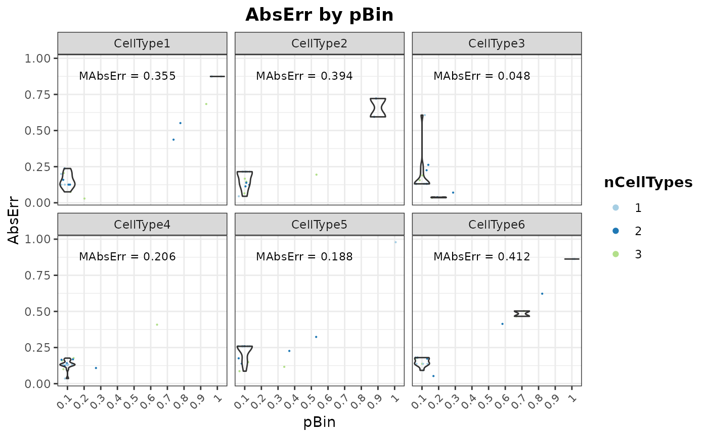
# representation, for more examples, see the vignettes
distErrorPlot(
  object = SDDLS,
  error = "AbsErr",
  facet.by = "CellType",
  color.by = "nCellTypes",
  error.label = TRUE
)
#> Warning: Groups with fewer than two data points have been dropped.
#> Warning: Groups with fewer than two data points have been dropped.
#> Warning: Groups with fewer than two data points have been dropped.
#> Warning: Groups with fewer than two data points have been dropped.
#> Warning: Groups with fewer than two data points have been dropped.
#> Warning: Groups with fewer than two data points have been dropped.
#> Warning: Groups with fewer than two data points have been dropped.
#> Warning: Groups with fewer than two data points have been dropped.
#> Warning: Groups with fewer than two data points have been dropped.
#> Warning: Groups with fewer than two data points have been dropped.
#> Warning: Groups with fewer than two data points have been dropped.
#> Warning: Groups with fewer than two data points have been dropped.
#> Warning: Groups with fewer than two data points have been dropped.
#> Warning: Groups with fewer than two data points have been dropped.
#> Warning: Groups with fewer than two data points have been dropped.

distErrorPlot(
  object = SDDLS,
  error = "AbsErr",
  x.by = "CellType",
  facet.by = NULL,
  color.by = "CellType",
  error.label = TRUE
)

# }

Generate box or violin plots showing error distribution

Usage

Arguments

Value

See also

Examples