Building new deconvoluion models: deconvolution of colorectal cancer samples
Source:vignettes/realModelWorkflow.Rmd
realModelWorkflow.RmdIn this example, we are going to reproduce the pre-trained model
DDLS.colon.lee available at the
digitalDLSorteRmodels R package. It was trained on data
from Lee et al. (2020) (GSE132465,
GSE132257
and GSE144735),
and consist of ~ 100,000 cells from a total of 31 patients including
tumoral and healthy samples. These cells are divided into 22 cell types
covering the main ones found in this kind of samples:
Anti-inflammatory_MFs (macrophages), B cells,
CD4+ T cells, CD8+ T cells, ECs
(endothelial cells), ECs_tumor, Enterocytes,
Epithelial cells, Epithelial_cancer_cells,
MFs_SPP1+, Mast cells,
Myofibroblasts, NK cells,
Pericytes, Plasma_cells,
Pro-inflammatory_MFs, Regulatory T cells,
Smooth muscle cells, Stromal cells,
T follicular helper cells, cDC (conventional
dendritic cells), and gamma delta T cells. The expression
matrix only contains 2,000 genes selected by
digitalDLSorteR when the model was created to save time
and RAM. Thus, in this example we will set the parameters related to
gene filtering to zero.
suppressMessages(library("SummarizedExperiment"))
suppressMessages(library("SingleCellExperiment"))
suppressMessages(library("digitalDLSorteR"))
suppressMessages(library("ggplot2"))
suppressMessages(library("dplyr"))

if (!requireNamespace("digitalDLSorteRdata", quietly = TRUE)) {
  remotes::install_github("diegommcc/digitalDLSorteRdata")
}
suppressMessages(library("digitalDLSorteRdata"))
suppressMessages(library("dplyr"))
suppressMessages(library("ggplot2"))
Loading data
We are also going to load bulk RNA-seq data on colorectal cancer patients from the The Cancer Genome Atlas (TCGA) program (Koboldt et al. 2012; Ciriello et al. 2015). When building new deconvolution models, we recommend loading both the single-cell RNA-seq reference and the bulk RNA-seq dataset to be deconvoluted at the beginning so that digitalDLSorteR can choose only those genes that are actually relevant for the both of them.
data("SCE.colon.Lee")
data("TCGA.colon.se")
# to make it suitable for digitalDLSorteR
rowData(TCGA.colon.se) <- DataFrame(SYMBOL = rownames(TCGA.colon.se))
DDLS.colon <- createDDLSobject(
  sc.data = SCE.colon.Lee,
  sc.cell.ID.column = "Index",
  sc.gene.ID.column = "SYMBOL",
  sc.cell.type.column = "Cell_type_6",
  bulk.data = TCGA.colon.se,
  bulk.sample.ID.column = "Bulk",
  bulk.gene.ID.column <- "SYMBOL",
  filter.mt.genes = "^MT-",
  sc.filt.genes.cluster = FALSE,
  sc.log.FC = FALSE,
  sc.min.counts = 0,
  sc.min.cells = 0,
  verbose = TRUE,
  project = "Colon-Cancer-Project"
)
## === Processing bulk transcriptomics data## - Removing 2568 genes without expression in any cell## - Filtering features:## - Selected features: 54918## - Discarded features: 1599## ## === Processing single-cell data## - Filtering features:## - Selected features: 2000## - Discarded features: 0##
## === No mitochondrial genes were found by using ^MT- as regrex##
## === Final number of dimensions for further analyses: 2000After loading the data, we have a DigitalDLSorter object
with 2,000 genes and both the single-cell RNA-seq used as reference and
the bulk RNA-seq data to be deconvoluted.
DDLS.colon## An object of class DigitalDLSorter
## Real single-cell profiles:
## 2000 features and 106364 cells
## rownames: RP1-276N6.2 RILPL1 SERPINA5 ... SERPINA5 LGMN CXCL11 PLA2G5
## colnames: SMC07-T_AGCATACGTGTGCCTG SMC22-T_CACACAATCCACGAAT SMC24-T_CACATTTAGCAGGCTA ... SMC24-T_CACATTTAGCAGGCTA SMC16-T_GTAGGCCTCGCCTGTT SMC03-N_CCATGTCAGAATTGTG SMC08-T_ACAGCCGAGTTGTCGT
## Bulk samples to deconvolute:
## Bulk.DT bulk samples:
## 2000 features and 521 samples
## rownames: NACAD NRXN1 FAM81A ... FAM81A COL3A1 RGS5 AURKC
## colnames: dc38ba64.6240.4bab.9ad5.2adb67e1b79e eb843ddf.f91d.4f04.b34c.549b1f53ee92 cf7ced35.7e29.4bdc.92e7.b56c315c54eb ... cf7ced35.7e29.4bdc.92e7.b56c315c54eb X3b8d04cd.d658.46ba.adca.079fee531e17 X574a3ef3.ea84.45f4.b20d.8b3d2b172793 X789c1767.4073.4ffa.b193.54b20b96d55e
## Project: Colon-Cancer-ProjectGenerating cell composition matrix
Now, let’s generate the cell composition matrix by using the
generateBulkCellMatrix function. It requires a data frame
with prior knowledge about how likely is to find each cell type in a
sample. For this example, we have used an approximation based on the
frequency of each cell type in each patient/sample from the scRNA-seq
dataset:
prop.design <- single.cell.real(DDLS.colon)@colData %>% as.data.frame() %>%
  group_by(Patient, Cell_type_6) %>% summarize(Total = n()) %>%
  mutate(Prop = (Total / sum(Total)) * 100) %>% group_by(Cell_type_6) %>%
  summarise(Prop_Mean = ceiling(mean(Prop)), Prop_SD = ceiling(sd(Prop))) %>%
  mutate(
    from = Prop_Mean,
    to.1 = Prop_Mean * (Prop_SD * 2),
    to = ifelse(to.1 > 100, 100, to.1),
    to.1 = NULL, Prop_Mean = NULL, Prop_SD = NULL
  )
## `summarise()` has grouped output by 'Patient'. You can override using the `.groups` argument.Then, we can generate the actual pseudobulk samples that will follow
these cell proportions. In this case, we generate 10,000 pseudobulk
samples (num.bulk.samples), although this number could be
increased according to available computational resources.
## for reproducibility
set.seed(123)
DDLS.colon <- generateBulkCellMatrix(
  object = DDLS.colon,
  cell.ID.column = "Index",
  cell.type.column = "Cell_type_6",
  prob.design = prop.design,
  num.bulk.samples = 10000,
  verbose = TRUE
) %>% simBulkProfiles(threads = 2)
##
## === The number of bulk RNA-Seq samples that will be generated is equal to 10000##
## === Training set cells by type:## - Anti-inflammatory_MFs: 501
## - B cells: 7336
## - CD4+ T cells: 10595
## - CD8+ T cells: 7570
## - cDC: 481
## - ECs: 874
## - ECs_tumor: 1398
## - Enterocytes: 920
## - Epithelial cells: 1411
## - Epithelial_cancer_cells: 19447
## - gamma delta T cells: 1459
## - Mast cells: 499
## - MFs_SPP1+: 4118
## - Myofibroblasts: 1789
## - NK cells: 1056
## - Pericytes: 677
## - Plasma_cells: 6259
## - Pro-inflammatory_MFs: 2342
## - Regulatory T cells: 4233
## - Smooth muscle cells: 614
## - Stromal cells: 5555
## - T follicular helper cells: 639## === Test set cells by type:## - Anti-inflammatory_MFs: 155
## - B cells: 2456
## - CD4+ T cells: 3515
## - CD8+ T cells: 2583
## - cDC: 163
## - ECs: 336
## - ECs_tumor: 431
## - Enterocytes: 347
## - Epithelial cells: 439
## - Epithelial_cancer_cells: 6400
## - gamma delta T cells: 499
## - Mast cells: 175
## - MFs_SPP1+: 1406
## - Myofibroblasts: 592
## - NK cells: 325
## - Pericytes: 206
## - Plasma_cells: 2075
## - Pro-inflammatory_MFs: 761
## - Regulatory T cells: 1467
## - Smooth muscle cells: 191
## - Stromal cells: 1829
## - T follicular helper cells: 240## === Probability matrix for training data:## - Bulk RNA-Seq samples: 7500
## - Cell types: 22## === Probability matrix for test data:## - Bulk RNA-Seq samples: 2500
## - Cell types: 22## DONE## === Setting parallel environment to 2 thread(s)##
## === Generating train bulk samples:##
## === Generating test bulk samples:##
## DONENeural network training
After generating the pseudobulk samples, we can train and evaluate the model. The training step is only performed using cells/pseudobulk samples coming from the training subset, since the test subset will be used for the assessment of its performance.
DDLS.colon <- trainDDLSModel(object = DDLS.colon, verbose = FALSE)##
1/79 [..............................] - ETA: 3s - loss: 0.1169 - accuracy: 0.7500 - mean_absolute_error: 0.0116 - categorical_accuracy: 0.7500
79/79 [==============================] - 0s 500us/step - loss: 0.1221 - accuracy: 0.7056 - mean_absolute_error: 0.0133 - categorical_accuracy: 0.7056
##
79/79 [==============================] - 0s 503us/step - loss: 0.1221 - accuracy: 0.7056 - mean_absolute_error: 0.0133 - categorical_accuracy: 0.7056Evaluation of the model on test data
Once the model is trained, we can explore how well the model behaves on test samples. This step is critical because it allows us to assess if digitalDLSorteR is actually understanding the signals coming from each cell type or if on the contrary there are cell types being ignored.
DDLS.colon <- calculateEvalMetrics(object = DDLS.colon)digitalDLSorteR implements different functions to visualize the results and explore potential biases on the models. For this tutorial, we will check the correlation between expected and predicted proportions, but for a more detailed explanation about other visualization functions, check the Documentation.
corrExpPredPlot(
  DDLS.colon,
  color.by = "CellType",
  facet.by = "CellType",
  corr = "both",
  size.point = 0.5
)
## `geom_smooth()` using formula = 'y ~ x'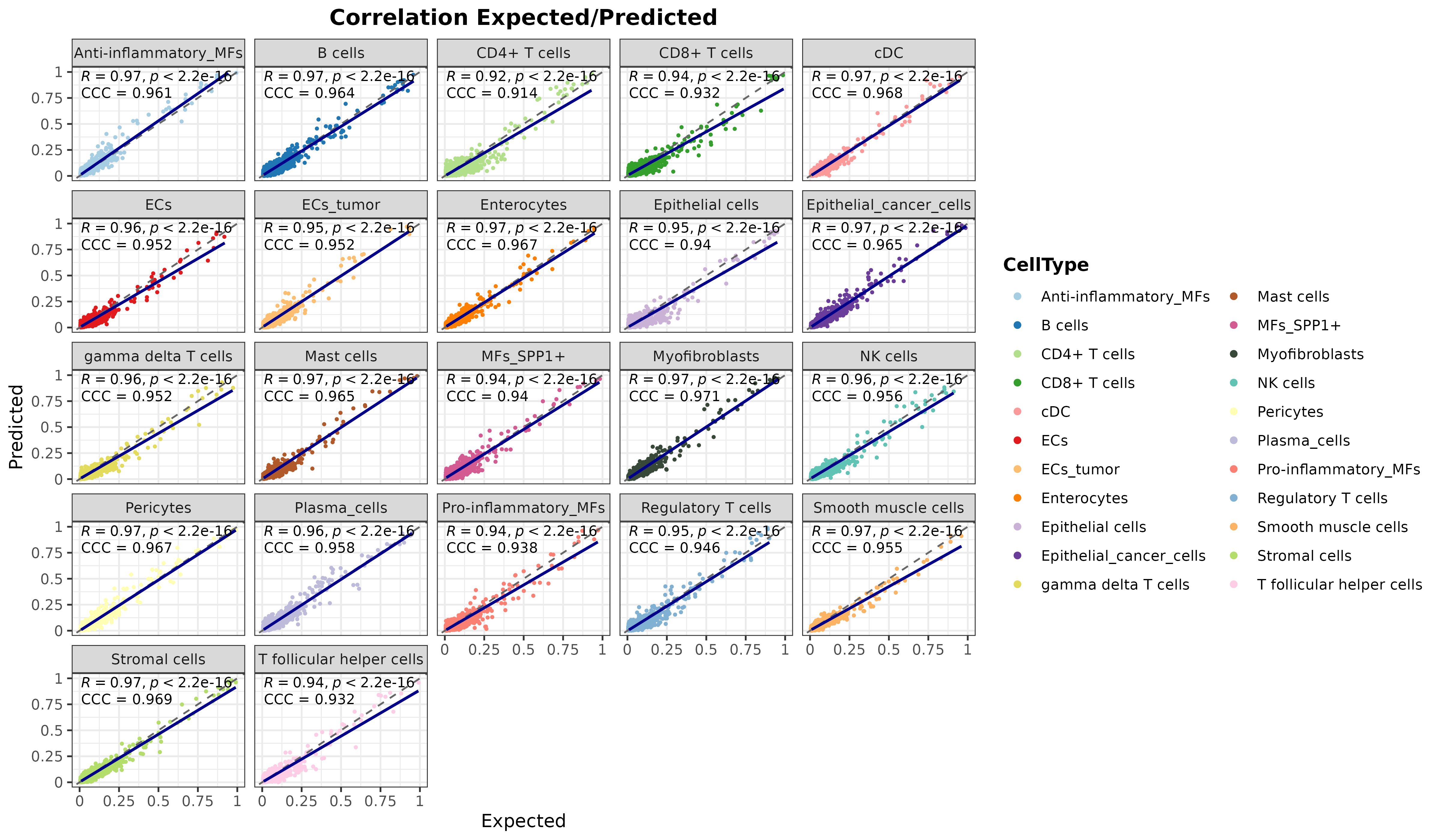
plot of chunk corr1_realModelWorkflow
As it can be seen, the model is accurately predicting the cell proportions of pseudobulk samples from the test data, which means that it is detecting differential signals for each cell type.
Deconvolution of TCGA samples
Now, to show its performance on real data, we are going to
deconvolute the samples from the TCGA project (Koboldt et al. 2012; Ciriello et al. 2015)
loaded at the beginning of the vignette. This dataset consists of 521
samples and includes both tumoral and healthy samples. This step is
performed by the deconvDDLSObj function, which will use the
trained model to obtain a set of predicted proportions for each sample
contained in the deconv.data slot.
DDLS.colon <- deconvDDLSObj(object = DDLS.colon, verbose = FALSE)## No 'name.data' provided. Using the first datasetWe can plot the results as follows:
barPlotCellTypes(DDLS.colon, rm.x.text = TRUE)## 'name.data' not provided. By default, first results are used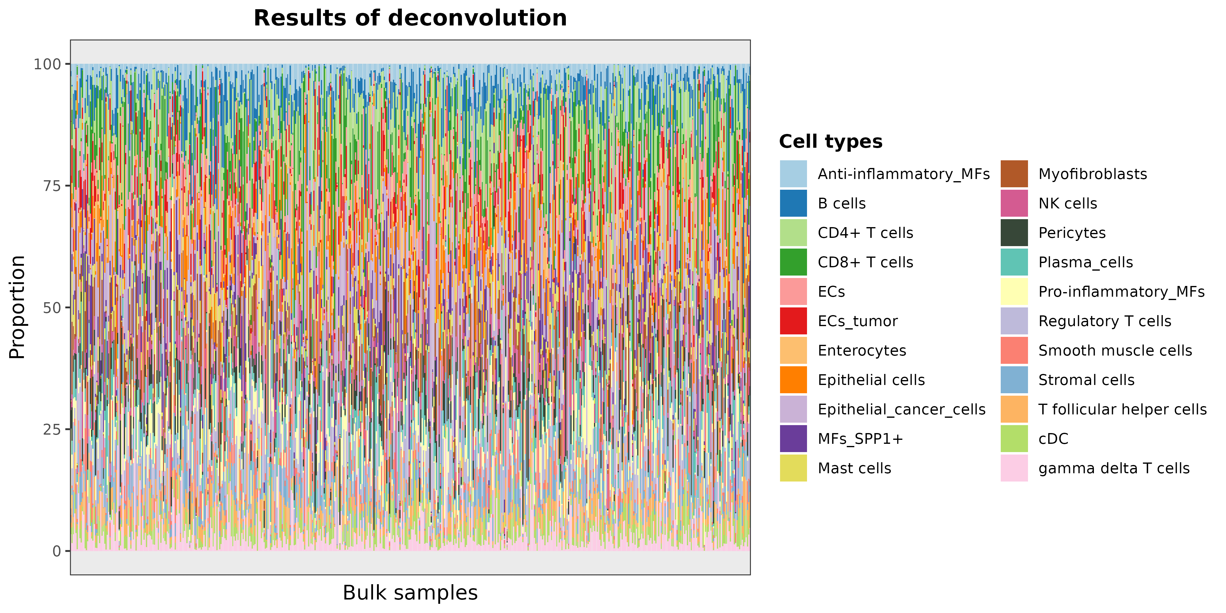
plot of chunk barPlotResults_realModelWorkflow
As the total number of samples is too high, we can see the results of
some samples by taking the predicted cell proportions and plotting 20
random samples with barPlotCellTypes:
set.seed(12345)
resDeconvTCGA <- deconv.results(DDLS.colon, name.data = "Bulk.DT")
barPlotCellTypes(
  resDeconvTCGA[sample(1:521, size = 20), ], rm.x.text = TRUE,
  title = "Results of deconvolution (20 random samples)"
)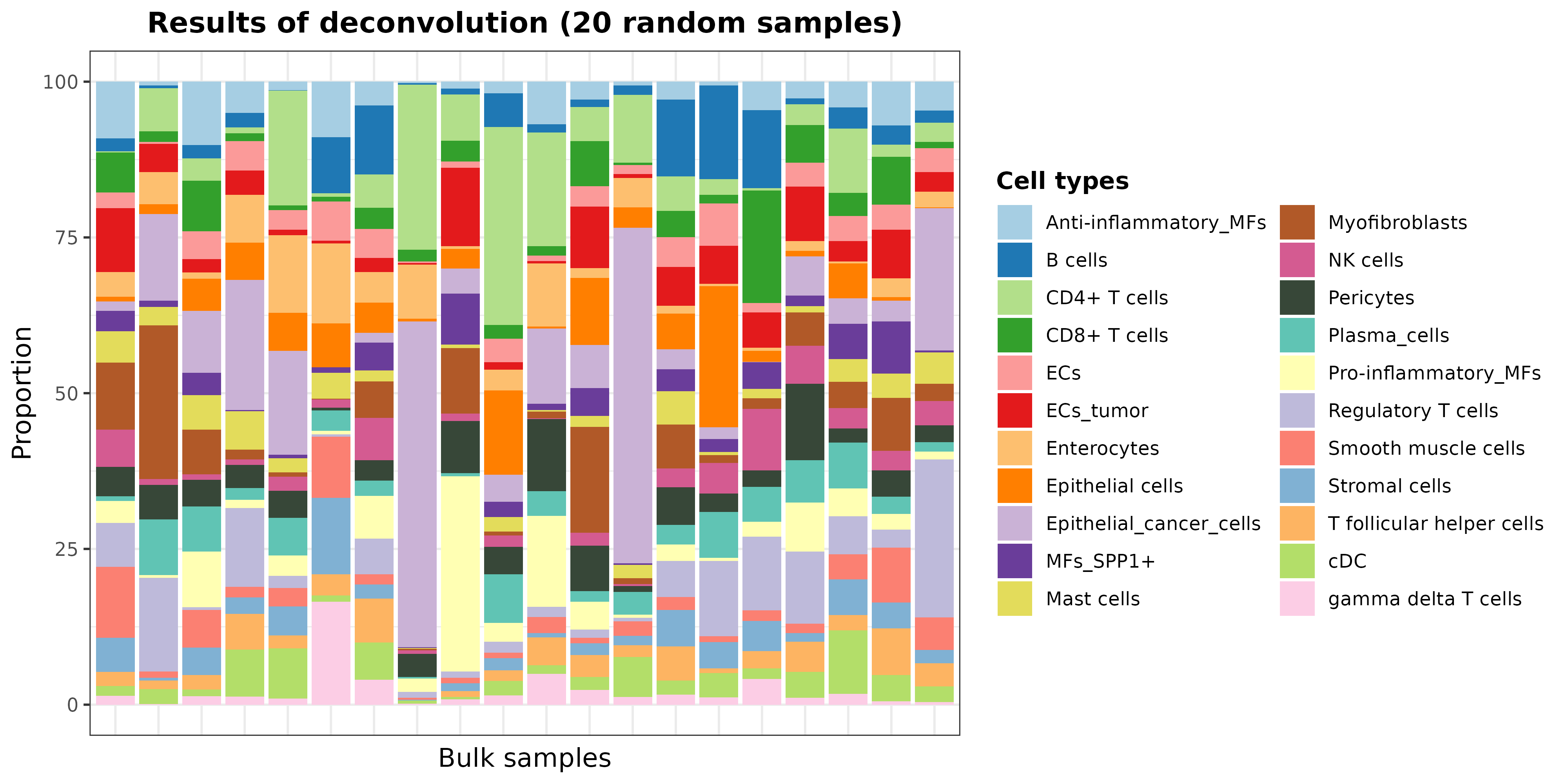
plot of chunk barPlotResults20_realModelWorkflow
Now, we can represent the cell proportions of every cell type
considered by the model separating healthy and tumoral samples. We are
also going to filter out samples considered metastatic or recurrent
(check the TCGA.colon.se object) because these groups are
composed of only 1 sample:
data.frame(
  Sample = rownames(resDeconvTCGA),
  TypeSample = colData(TCGA.colon.se)[["Tumor_Type"]]
) %>% cbind(resDeconvTCGA) %>%
  reshape2::melt() %>% filter(!TypeSample %in% c("Metastatic", "Recurrent")) %>%
  ggplot(aes(x = TypeSample, y = value, fill = variable)) +
  geom_boxplot() + facet_wrap(~ variable, scales = "free") +
  scale_fill_manual(values = digitalDLSorteR:::default.colors()) +
  ggtitle("Estimated proportions in TCGA data (all cell types)") + theme_bw() +
    theme(
      plot.title = element_text(face = "bold", hjust = 0.5),
      legend.title = element_text(face = "bold")
    )
## Using Sample, TypeSample as id variables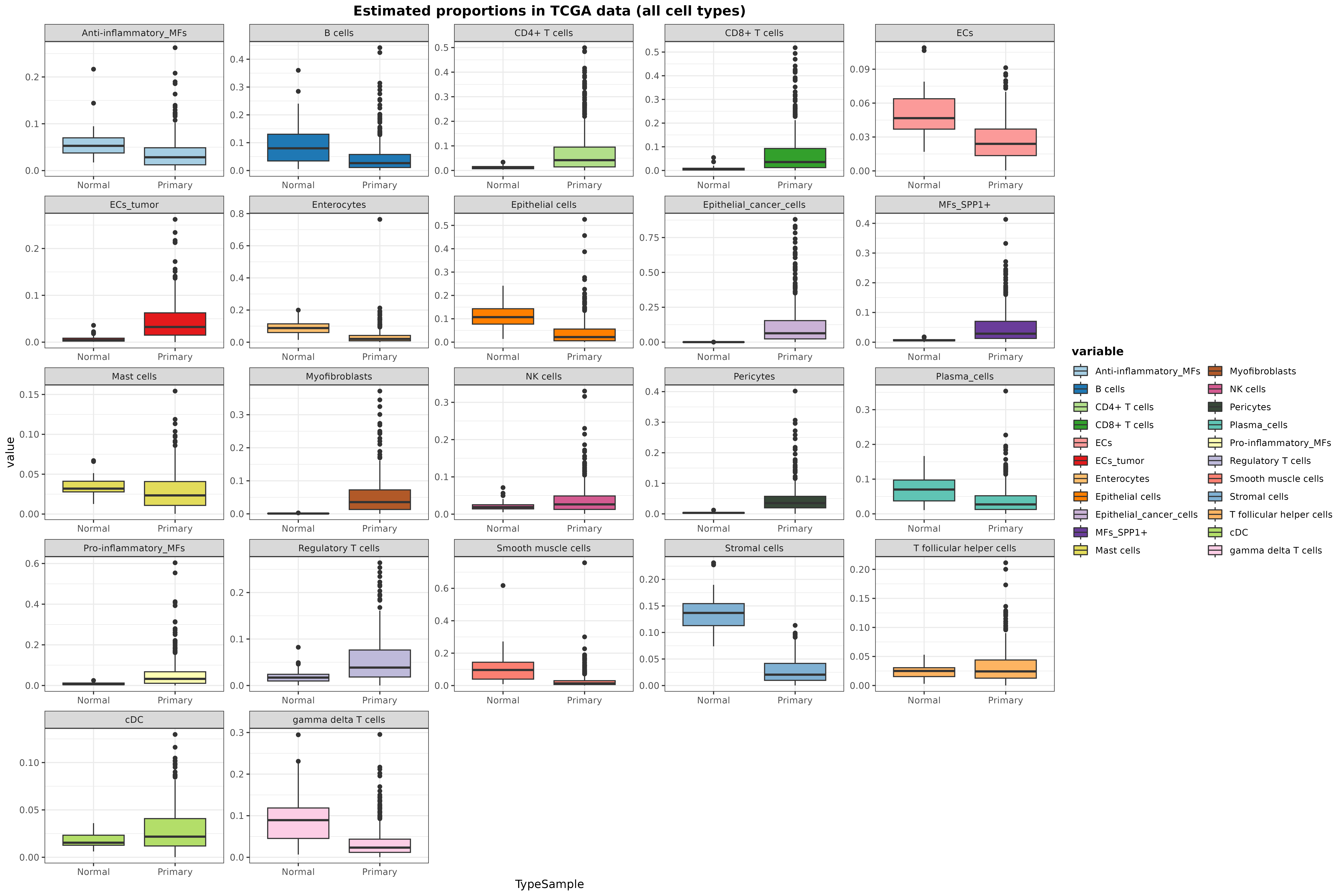
plot of chunk boxplotResults_realModelWorkflow
In general, the results seem to be in line with what it is known: tumoral samples show a huge immune infiltration, whereas other cell types such as epithelial cells are displaced. We can also specifically inspect the predicted proportions of enterocytes, tumor, epithelial, and stromal cells:
data.frame(
  Sample = rownames(resDeconvTCGA),
  CRC = resDeconvTCGA[, "Epithelial_cancer_cells"],
  Epithelial = resDeconvTCGA[, "Epithelial cells"],
  Stromal = resDeconvTCGA[, "Stromal cells"],
  Entero = resDeconvTCGA[, "Enterocytes"],
  TypeSample = TCGA.colon.se@colData$Tumor_Type
) %>% filter(!TypeSample %in% c("Metastatic", "Recurrent")) %>%
  reshape2::melt() %>%
  ggplot(aes(x = TypeSample, y = value, fill = TypeSample)) +
    geom_boxplot() + facet_wrap(~ variable) + ylab("Estimated proportion") +
  scale_fill_manual(values = digitalDLSorteR:::default.colors()) +
    ggtitle("Estimated proportions in TCGA data") + theme_bw() +
    theme(
      plot.title = element_text(face = "bold", hjust = 0.5),
      legend.title = element_text(face = "bold")
    )
## Using Sample, TypeSample as id variables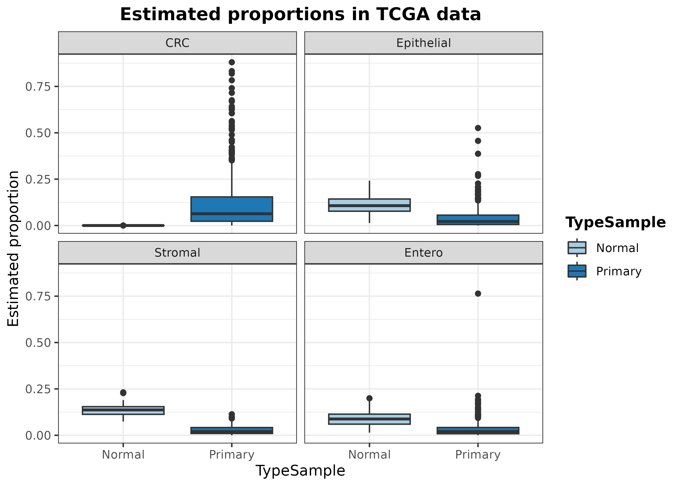
plot of chunk boxplotResults_2_realModelWorkflow
As it can be seen, digitalDLSorteR correctly
estimates the absence of tumor cells (CRC) in healthy
samples. On the other hand, the predicted proportion of enterocytes,
epithelial and stromal cells decrease in the tumoral samples, which
makes sense considering the infiltration of immune cells and the
increased presence of tumoral cells.
Interpreting the neural network model
Finally, we have implemented a way to make the predictions made by digitalDLSorteR more interpretable. This part was developed for our new R package for deconvolution of spatial transcriptomics data SpatialDDLS, and the methodology is explained in Mañanes et al. (2024).
DDLS.colon <- interGradientsDL(DDLS.colon)We can explore the top 5 genes with the highest gradient for each cell type to check which genes are being more used by the model:
top.gradients <- topGradientsCellType(
  DDLS.colon, method = "class", top.n.genes = 5
)
sapply(
  top.gradients, \(x) x$Positive
) %>% as.data.frame()
## Anti-inflammatory_MFs B cells CD4+ T cells CD8+ T cells ECs ECs_tumor Enterocytes
## 1 LYVE1 IGHD KLRB1 GZMK FABP5 INSR UGT2B17
## 2 PLTP CD19 ANXA1 GZMH SOCS3 AQP1 ITM2C
## 3 FOLR2 FCRL1 GPR183 ITM2C CD36 HSPG2 UGT2A3
## 4 PDK4 PAX5 MAL VCAM1 CD320 IGFBP5 PCSK1N
## 5 RNASE1 CD83 LTB NKG7 SLC14A1 FKBP1A MYOM1
## Epithelial cells Epithelial_cancer_cells MFs_SPP1+ Mast cells Myofibroblasts NK cells
## 1 ZG16 AREG CTSD ANXA1 LGALS1 FGFBP2
## 2 AQP8 PLTP APOC1 GATA2 RP11-400N13.3 CMC1
## 3 URAD EN2 RP11-1008C21.1 CTSG ITM2C GNLY
## 4 TFF3 CTSH GPNMB VIM IGFL2 KRT86
## 5 REP15 GSTP1 APOE LMNA RP11-54O7.3 KLRC1
## Pericytes Plasma_cells Pro-inflammatory_MFs Regulatory T cells Smooth muscle cells Stromal cells
## 1 CD36 LINC00152 FCN1 BATF RERGL EPHA7
## 2 LINC00152 RGS1 S100A12 RTKN2 CASQ2 FCGRT
## 3 MAP6 IGHA1 TIMP1 TNFRSF4 DES C7
## 4 RNF152 IGHV4-61 IL1RN IL32 SNCG SEMA3E
## 5 CNTN4 SRGN SERPINB2 LTB RBM24 ZFP36
## T follicular helper cells cDC gamma delta T cells
## 1 CXCL13 HLA-DQA2 KLRC2
## 2 NR3C1 INSIG1 TRGC2
## 3 NMB CST7 TRDC
## 4 PTPN13 CD1C CCL5
## 5 SRGN ENHO GZMAIn addition, digitalDLSorteR also implements a function to plot the top gradients per cell type as a heatmap:
hh <- plotHeatmapGradsAgg(DDLS.colon, top.n.genes = 4, method = "class")
hh$Absolute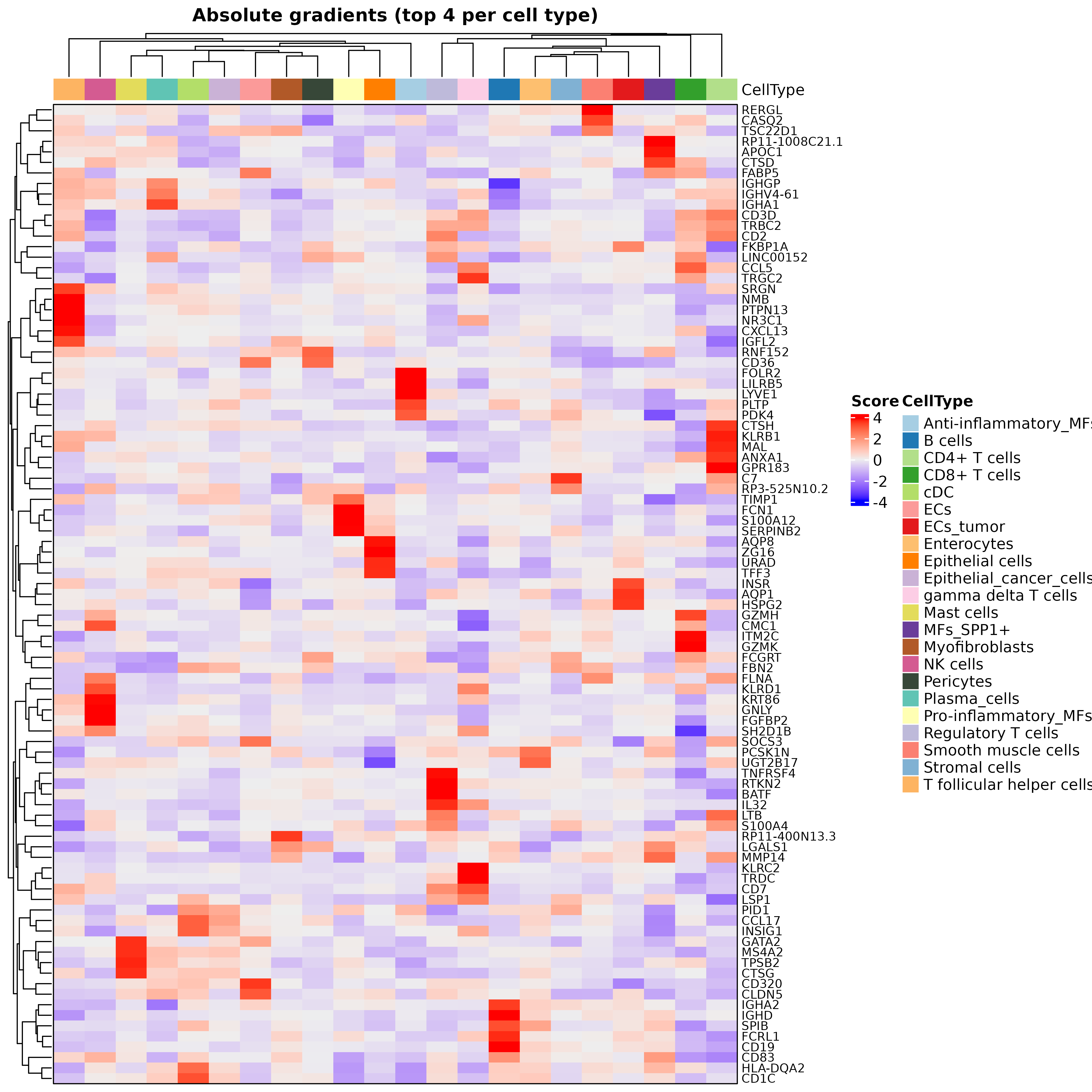
plot of chunk heatmapGradients_realModelWorkflow
It is important to note that these markers should not be interpreted as cell type markers. Rather, they serve as indications to help interpret the model’s performance. In addition, due to the multivariate nature of this approach, gradients are surrogates at the feature level for predictions made considering all input variables collectively, and thus caution should be exercised in drawing direct conclusions about specific gene-cell type relationships.